[Improving Deep Neural Networks] week3. Hyperparameter tuning, Batch Normalization and Programming Frameworks

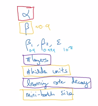
Hyperparameter parameters

Tips for hyperparam-tuning.

Tuning process

Many hyperparams to tune, mark importance by colors (red > yellow > purple):

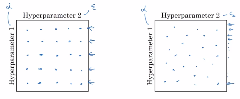
How to select set of values to explore ?

• Do NOT use grid search (grid of n * n)

— this was OK in pre-DL era.

• try random values.

reason: difficule to know which hyperparam is most important, by randomization, can try out nn distinct values for each hyperparam.*
In extreme case, one is alpha, the other is epislon.

• in grid search: only n distinct values of alpha are tried
• in random choice: can have n*n distinct values of alpha

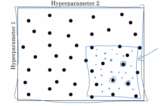
• Coarse to fine sample scheme: zoom in to smaller regions of hyperparam space and re-sample more densely.

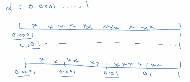
Using an appropriate scale to pick hyperparameters

"Sampling at random", but at appropriate scale, not uniformly.
example: choice of alpha in [0.001, 1]
→ sample uniformly at log scale is more resonable: equal resources are used to search at each scale.

implementation:

r = -4 * np.random.rand()  # -4 <= r <= 0, uniformly at randome  
alpha = np.exp(10, r) # 10e-4 <= alpha <= 1.0

sampling beta for exp-weighted-avg: sample in the range of [0.9, 0.999]
→ convert to sampling 1-beta, which is in range [0.0001, 0.1]

Hyperparameters tuning in practice: Pandas vs. Caviar

Tricks on how to organize hyper-param-tuning process.

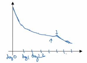
re-test hyperparams occasionally: intuitions get stale, re-evaluate hyperparams every several months.

Two major schools of training

• Panda approach: babysitting one model

Huge dataset, limited computing resources, can only train one model → babysit the model as it's training. Watch learning curve, try changing hyparams once a day.

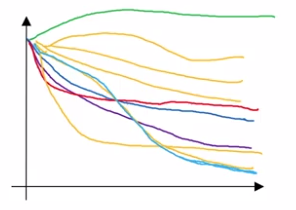
• Caviar approach: train many models in parallel

Have enough computation power.
Different model/hyperparams being trained at the same time in parallel, pick the best one.

Batch Normalization

Batch normalization:
(in some cases) makes NN much more robust, and DNN much easier to train.

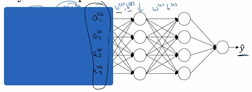
Normalizing activations in a network

In pre-DL: normalize inputs to speedup learning. "make contours round"

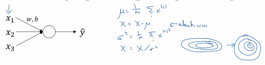
In NN: normalize the activation a[l-1] from previous layer could help (in practice, usually normalize z[l-1].)

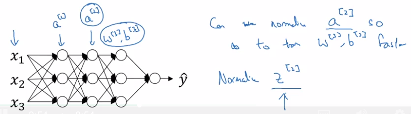
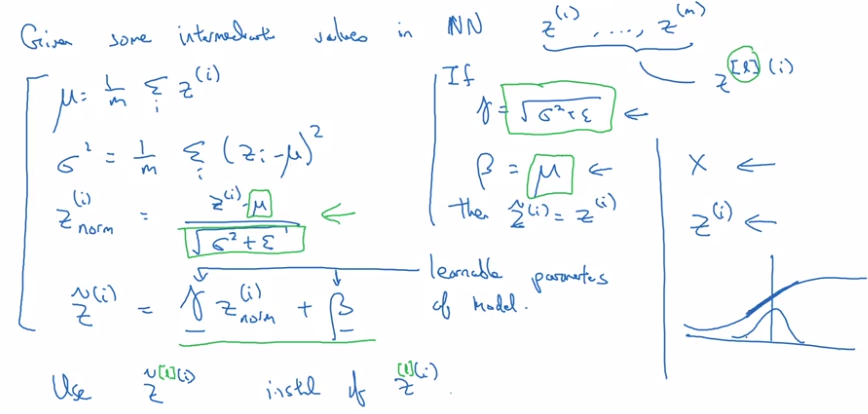
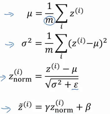
BatchNorm algo:
intermediate values at each layer: z[l]
→ compute mean & variance
⇒ get normalized z[l]_normed. (mean=0, std=1)
→ trasform z[l]_normed to z_tilde[l] (mean=beta, std=gamma, beta and gamma are learnable params),
reason: for hidden units, want to move/stretch the support of hidden inputs, so as to profit from non-linearity of activation function.

Fitting Batch Norm into a neural network

Add batchnorm to NN: replace z[l] to z_tilde[l] at each layer before activation g[l].

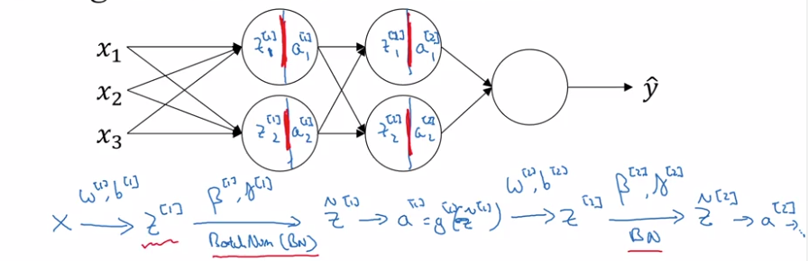
Extra params to learn: gamma[l] and beta[l] at each layer.

In practice: no need to implement all details of BN, use DL framework.

No bias term (b) in BN:
z[l] = W[l] * a[l-1] + b[l]
but z[l] will be centered anyway → b[l] is not useful.
→ b[l] is replaced by beta[l]

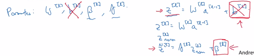
Dimension of beta[l], gamma[l]: the same as b[l] ( = n[l] * 1).

Why does Batch Norm work?

intuition 1: similar to normalizing input ("make contours round")

intuition 2: weights in deeper layers are more robust to changes in ealier layer weights.
i.e. Robost to data distribution changing. ("covariant shift")

motivating example:
cat-classification, trained all with black cats, but applied to colored cats.

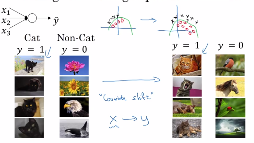
For NN, consider the 3rd layer's units:
input features: a[2],
if cover the first 2 layers, this is a NN to map from a[2] to y_hat
⇒ but when weights w[2],b[2] are updated in GD, a[2]'s distribution is always changing.

intuition: With BN, a[2] are ensured to always have the same mean/variance
→ "data distribution" is unchanged → later layers can learn more easily, independent of previous layer's weights' change.

intuition 2: BN as regularization
each minibatch is scaled by mean/var of just that minibatch
→ add noise to the transformation from z[l] to z_tilde[l].
⇒ similar to dropout, add noise to each layer's activations.
therefore BN have (slight) regularization effect (thie regularization effect gets smaller as minibatch size grows).
(This is an unintended side effect.)

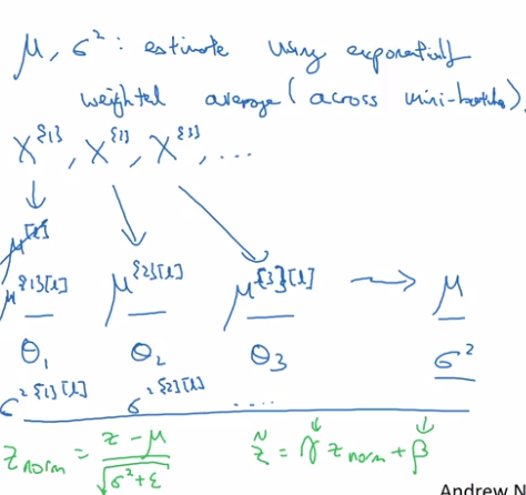
Batch Norm at test time

At training time, z[l] is standarlized over each minibatch.

⇒ But at test time needs to treat examples one at a time.
→ estimate the value of meu/sigma2
⇒ using exp-weighted-avg estimator across minibatchs (with beta close to 1 → ~running average).
at test time, just use the latest value of this exp-weighted-avg estimation as meu/sigma2.

Multiclass classification

Softmax Regression

So far: only binary classification
generalize logistic regression to >2 classes ⇒ softmax regression.

C = #classes, = #units in output layer
each component in y_hat is probability of one class, y_hat is normalized.

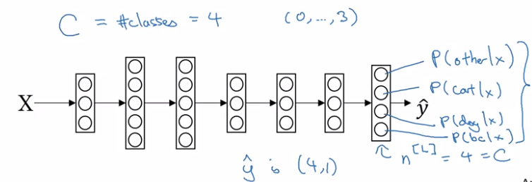
softmax layer:

• z[L] = W[L] * a[l-1] + b[L] — same as before
• a[L] = y_hat = g(z[L])

activation function: softmax
take exp(z[L]) --element-wise, and then normalize:

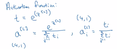
The softmax activation function is unusual because it takes a vector instead of scalar.
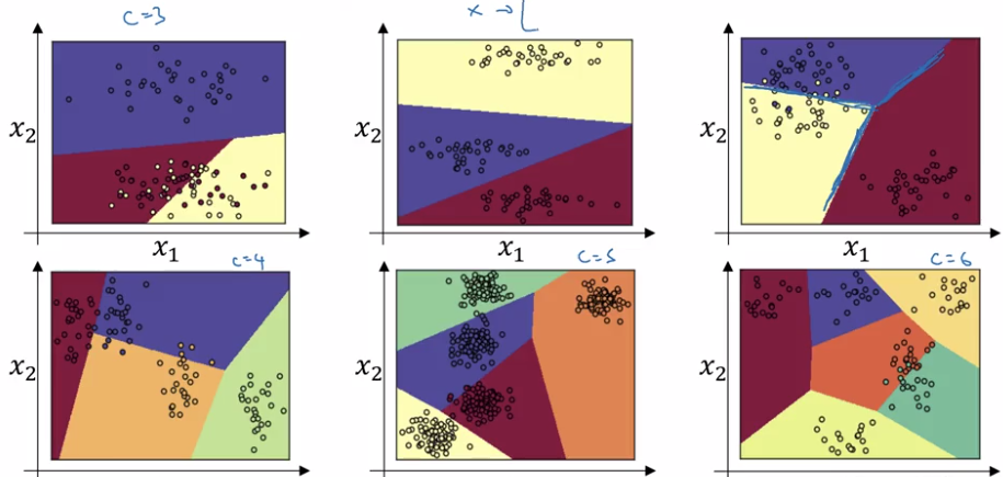
Softmax is generalization of logistic regression: decision boundary of a single-layer (no hidden layer) softmax is also linear:

Training a softmax classifier

understanding softmax

• "softmax" is in contrast to "hardmax":

hardmax[i]= 1 if z_i=max else 0.

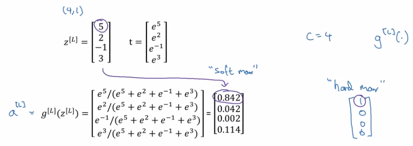
• When C = 2, softmax reduces to logistic regression.

softmax(C=2) = [logistic-reg(), 1-logistic-reg]

loss function
recall: loss function in logistic regression
L(y, y_hat) = -1 * sum( y_i * log yhat_i + (1-y_i) * log(yhat_i) )
→ want y_hat big when y_i=1, small when y_i=0

• training label y: one-hot encoding.
• prediciton y_hat: probability vector

loss function:

• if y_k=1, want to make yhat_k big

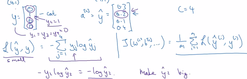
→ max-likelihood estimation.

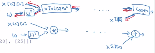
GD with softmax
fwdprop:
Z[L] --(softmax)--> a[L]=y_hat → L(y_hat, y)
backprop:
dZ[L] = y_hat - y

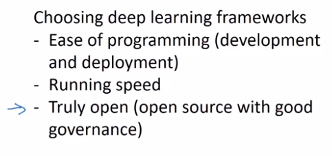
Introduction to programming frameworks

Deep learning frameworks

TensorFlow

motivating problem: minimize cost function J(w) = (w-5)^2

• import tensorflow as tf

• define parameter to optimize:
  w = tf.Variable(0, dtype=tf.float32)

• define cost function:
  cost = tf.add(tf.add(w**2), tf.multiply(-10., w)), 25) # w^2 - 10w + 25 # also possible to use tf-reloaded operators: cost = w**2 - 10 * w + 25

• tells tf to minimize the cost with GD optimizer:

train = tf.train.GradientDescentOptimizer(0.01).minimize(cost)
till now the computation graph is defined → backward derivatives are auto-computed.

• start the training

Quite idiomatic process:
initialize vars → create session → run operations in session

init = tf.global_variables_initializer()  
session = tf.Session()  
session.run(init)  
session.run(train) # run 1 iteration of training

alternative format:

with tf.Session() as session:  
  session.run(init)  
  session.run(train)

• To inspect the value of a parameter: print(session.run(w))

• Run 1000 iters of GD:

  for i in range(1000): session.run(train)

Let loss function depends on training data:

• define training data as placer holder.
  a placerholder is a variable whose value will be assigned later.
  x = tf.placeholder(tf.float32, [3,1]) cost = x[0][0] * w**2 + x[1][0] * w + x[2][0]

• feed actual data value to placerholder: use feed_dict in session.run()

  data = np.array([1., -10., 25.]).reshape((3,1) session.run(train, feed_dict={x: data})