Setting up your Maching Learning Application
Train / Dev / Test sets
Applied ML: highly iterative process. idea-code-exp loop
splitting data
splitting data in order to speed up the idea-code-exp loop:
*training set / dev(hold-out/cross-validataion) set / test set *
split ratio:
- with 100~10000 examples: 70/30 or 60/20/20
- with ~1M examples: dev/test set can have much smaller ratio, e.g. 98/1/1
mismatched train/test distribution
training and test set don't come from the same dist.
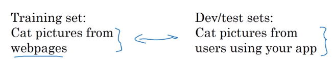
- rule of thumb: make sure dev and test set come from the same distribution.
- might be OK to only have dev set. — thought in this case no longer have unbiased estimate of performance.
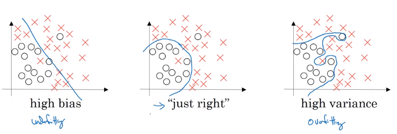
Bias / Variance
- high variance: overfitting
- high bias: underfitting
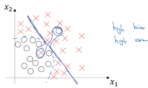
high base and high variance (worse case): high bias in some region and high variance elsewhere
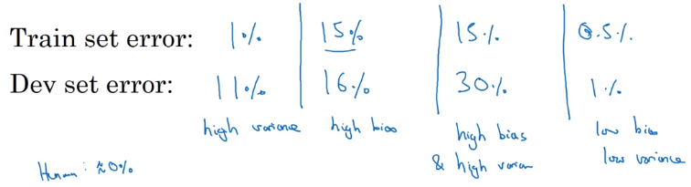
how to estimate bias&variance
→ look at train and dev set error
- high variance: Err_train << Err_dev — not generalize well
- high bias: Err_train ~= Err_dev, and Err_train >> Err_human — not learning well even on training set
- high bias and high variance (worse): Err_train >> Err_human, Err_train >> Err_dev
Basic Recipe for Machine Learning
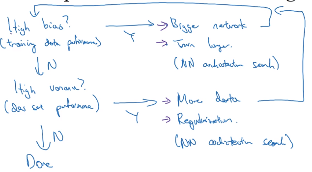
basic recipe:
- does algo have high bias ? (look at Err_train)
- if yes → try bigger nn / other architecture
- until having low bias (fit well training set)
- high variance ? (look at Err_dev)
- if yes → get more data / regularization / other architecture
bias-variance tradeoff
- in pre-DL era, bias and variance are tradeoff (decrease one → increase the other)
- in DL era: if getting bigger nn and more data always possible, both can be reduced
(when well regularized,) "training a bigger NN almost never hurts."
Regularizing your neural network
2 ways to reduce variance: regularize, or get more data.
Regularization
example: logistic regression
- params:
w,b - cost function
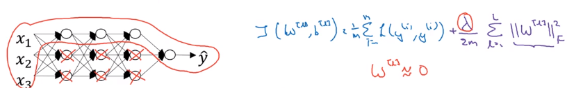
J(w,b) = 1/m * L(yhat_i, yi)
→ add one more term to cost J: adding L2 norm of w(L2 regularization)
(lambda: regularization param)
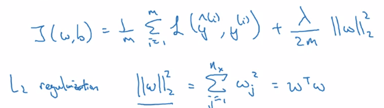
just omit regularizing b: w is high dim, b is single number.
L1 regularization: L1 norm of w → w will be sparse → compressing the model (just a little bit)
⇒ L2-reg is much often used
example: NN
- params:
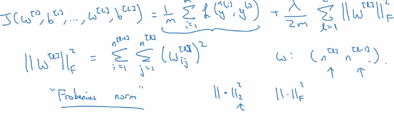
w[l],b[l]for l = 1..N - sum of the norms of each
w[l]matrix.
⇒ "Frobenius norm" of a matrix: sum (each element squared)
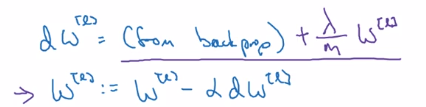
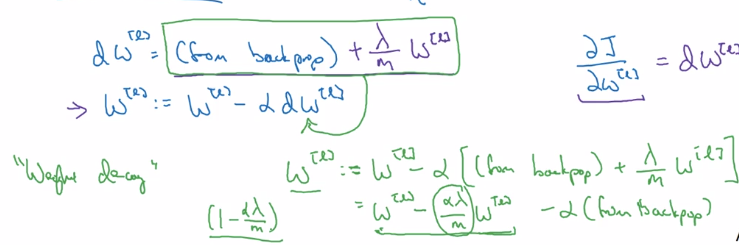
gradient descent: adding one more term from backprop
d(1/2m * ||w||) = lambda / m
L2-reg also called "weight decay":
with L2-reg, looks as if doing the backprop updating, with w being w' = (1-alpha*lambda/m) * w (decayed w)
Why regularization reduces overfitting?
why imposing small params prevents overfitting?
intuition 1
→ heavy regularization
→ weight ~= 0
→ many hidden units' impact are "zeroed-out"
→ simpler NN
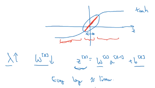
intuition 2
e.g. activation g(z) = tanh(z)
small z → g(z) ~= linear,
large z → g(z) flattend
⇒ large lambda → small w
→ z small
→ every layer ~linear
Dropout Regularization
another powerful method of regularization
dropout: For each training example, in each layer, eliminate randomly some of its output values.
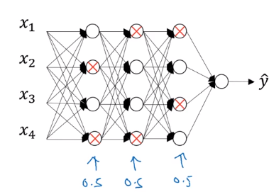
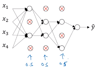
dropout implementation: "inverted dropout"
example: dropout of layer 3, keep_prob = 0.8 (prob of keeping hidden unit)
→ generate a rand matrix of shape the same shape as activation a[3]
d3 = np.random.rand(a3.shape[0], a3.shape[1]) < keep_prob  # d3 is bool matrix
a3 = np.multiply(a3, d3)  # element-wise multiply
a3 /= keep_prob  # ****"inverted dropout"****
"inverted dropout": why a3 /= keep_prob (i.e. make a3 larger)?
- let's say layer 3 has 50 units, keep_prob = 0.8
- → ~10 units shut off
z[4] = w[4] * a[3] + b[4]
⇒ a[3] have random 20% units shut off
→ w[4]a[3] will be reduced by 20% in expection*
- inverted dropout: a3 /= keep_prob, to keep expected value a3 remains unchanged.
- (No dropout at test time) → inverted dropout avoids scaling problem at test time
making predictions at test time
NOT use dropout at test time ⇒ don't want output to be random at test time...
Understanding Dropout
why randomly shut units prevents overfitting ?
Intuition: can't rely on any one input feature → have to spread out weight
spread weights ~→ smaller L2 norm (shrink weights)
Can be formally proven: dropout is equal to adaptive L2-reg, with penalty of different weight being different.
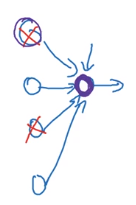
For one hidden unit: any of it input features (from prev layer) can go out at random
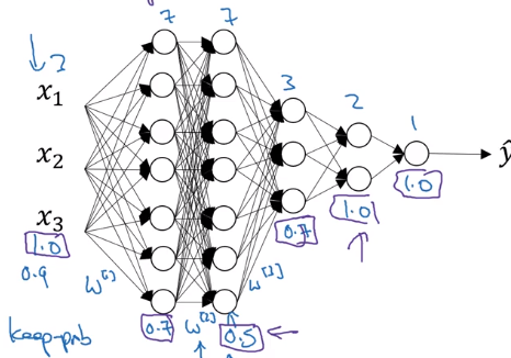
Implementation details
- vary keep_prob for different layer
→ smaller keep_prob for larger layer
- usually no dropout (or very small dropout) for input layer...
Downside of dropout
cost function J no longer well-defined (because output yhat is random)
→ can no longer plot cost-iter curve
→ turn off dropout before plotting the curve
Other regularization methods
data augmentation
adding more training example is expensive
→ vary existing training data (e.g. flipping/rand-distortions of training image for cats)
early stopping
plot Err or J to #iterations for both train and dev set.
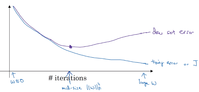
Downside of early-stopping:
optimization cost J and not overfitting should be separated task ("Orthogonalization")
→ early-stopping couples the two jobs.
upside of early stopping: no need to try different values of regularization param (lambda) → finds "mid-size w" at once.
Setting up your optimization problem
How to speed up training (i.e. optimize J)
Normalizing inputs
normalize input:
- substract mean
- normalize variance
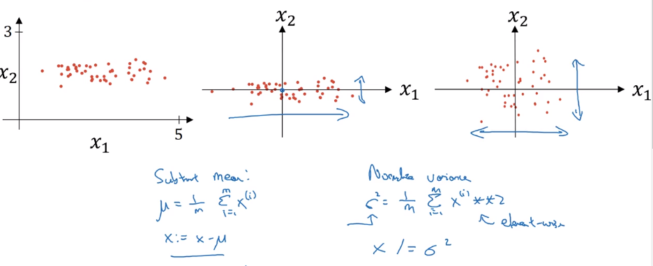
detail: in data splitting, use the same meu/sigma to normalize test set !
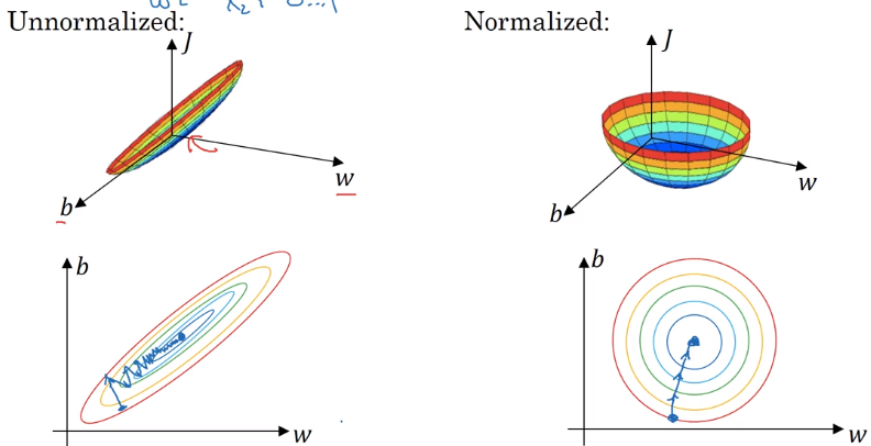
why normalizing input ?
if features x1 x2 are on different scales → w1 and w2 not same scale
J is more symmetric, easier to optimize
Vanishing / Exploding gradients
One problem in training very deep NN: vanishing/exploding gradients.
example: a very deep NN, each layer 2 units, linear activation g(z)=z, ignore bias b[l] = 0.
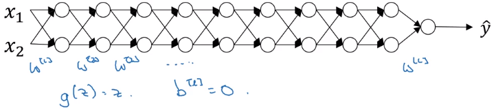
linear activations → y is just a linear transformation of x
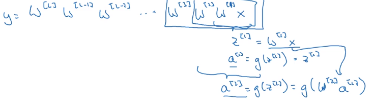
- assuming each w[l] = 1.5 * Identity_matrix ⇒ activations increase exponentially
- assuming each w[l] = 0.5 * Id ⇒ activations decrease exponentially
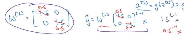
yhat too large or too small → hard to train
Weight Initialization for Deep Networks
A partial solution of vanishing/exploding gradient problem: carefully initialize weights.
single neuron example:
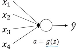
- y = g(w*x), g = relu
- n = # inputs for
z = w1x1 + ... + wnxn,
if wi are initzed randomly
→ large ns ⇒ z will be large !
⇒ set var(wi) = 1/n (2/n in practice) to keep z in similar scale for diffent #inputs
initialization code:
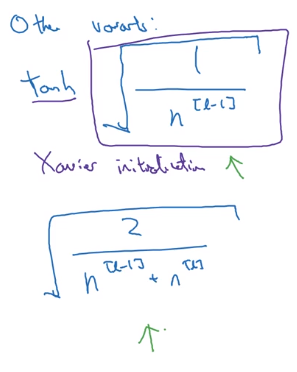
w[l] = np.random.randn(shape[l]) * np.sqrt( 2 / n[l-1] ) # n[l-1] = #inputs for layer-l
other variants
when activation function g = tanh
⇒ use var(wi) = 1/n ("Xavier initialization")
Numerical approximation of gradients
checking the derivative computation
example: f(x) = x ^ 3
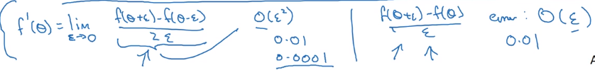
→ vary x by epsilon to approximate f'(x), use 2-sided difference
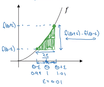
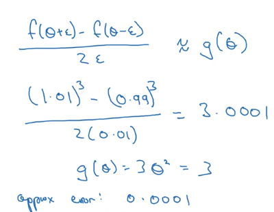
error order = O(epsilon^2) for 2-sided difference
Gradient checking
Verify that your implementation is correct. — help finding out bugs in implementation early.
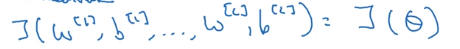
- concat all params into a big vector
theta - concat all dW[l] db[l] into big vector
d_theta - to check if d_theta is correct: construct a
d_theta_approxvector
⇒
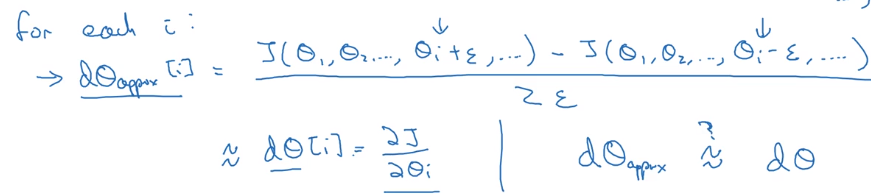
How to check "approximate":
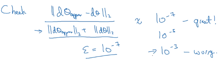
Gradient Checking Implementation Notes
- Dont' use checking in training: constructing d_theta_approx is slow
- When check fails: look at components to try to find bug
- Remember regularization: J contains reg term as well
- Doesn't work with dropout: J not well defined (random variable), turn dropout off before checking.
- Run check at random initialization (w,b~=0), then again after some training(w,b~>0)
Part 5 of series «Andrew Ng Deep Learning MOOC»:
- [Neural Networks and Deep Learning] week1. Introduction to deep learning
- [Neural Networks and Deep Learning] week2. Neural Networks Basics
- [Neural Networks and Deep Learning] week3. Shallow Neural Network
- [Neural Networks and Deep Learning] week4. Deep Neural Network
- [Improving Deep Neural Networks] week1. Practical aspects of Deep Learning
- [Improving Deep Neural Networks] week2. Optimization algorithms
- [Improving Deep Neural Networks] week3. Hyperparameter tuning, Batch Normalization and Programming Frameworks
- [Structuring Machine Learning Projects] week1. ML Strategy (1)
- [Structuring Machine Learning Projects] week2. ML Strategy (2)
- [Convolutional Neural Networks] week1. Foundations of Convolutional Neural Networks
- [Convolutional Neural Networks] week2. Deep convolutional models: case studies
- [Convolutional Neural Networks] week3. Object detection
- [Convolutional Neural Networks] week4. Special applications: Face recognition & Neural style transfer
- [Sequential Models] week1. Recurrent Neural Networks
- [Sequential Models] week2. Natural Language Processing & Word Embeddings
- [Sequential Models] week3. Sequence models & Attention mechanism
Disqus 留言