[Convolutional Neural Networks] week4. Special applications: Face recognition & Neural style transfer

This week: two special application of ConvNet.

I-Face Recognition

What is face recognition

Face verification & face recognition

• verification: input = image and ID → output whether the image and ID are the same.
• recognition: database = K persons, input = image → output = ID of the image among the K person or "not recognized".

→ the verification system's precision needs to be very high in order to be used in face recognition.

One Shot Learning

"one shot": learn from just one example, and able to recognize the person again.
A CNN+softmax is not practical, e.g. when new images are added to database, output_dim will change...

⇒ instead, learn a similarity function.
d(img1, img2) = degree of difference between images. + threshold tau

Siamese Network

To learn a disimilarity function: Siamese Network.

Use CNN+FC to encode a pic x into vector f(x).

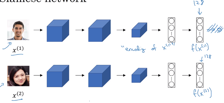
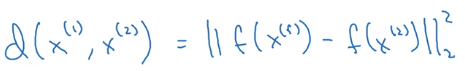
⇒ define disimilarity function d(x1, x2) as distance between encoded vectors.

More formally:
want to learn NN params for the encoding f(x) such that:
when x1 and x2 are same person, dist(f(x1), f(x2)) is small, otherwise large.

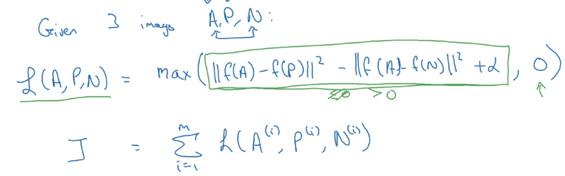
Triplet Loss

triplet: (anchor, positive, negative).

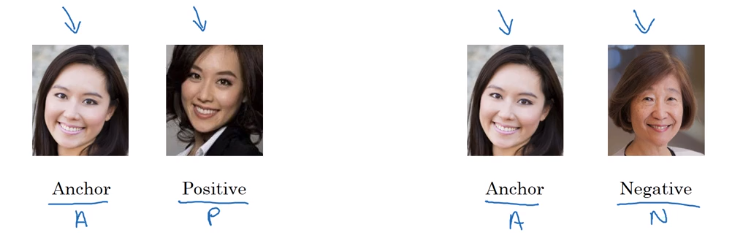
want f(A) similar to f(P) and different from f(N):
i.e. want d(A, P) - d(A, N) <= 0
⇒ to avoid NN from learning a trival output (i.e. all encodings are identical, d(A, P)=d(A, N)=0), add margin alpha.
want d(A, P) - d(A, N) + alpha<= 0

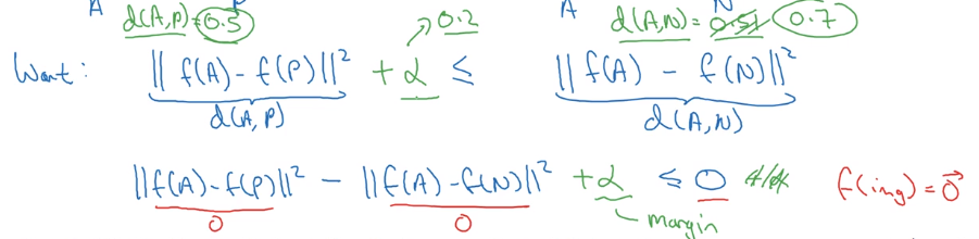
Loss function definition:
similar to hinge loss: L = max(0, d(A,P)-d(A,N) + alpha)

→ Generate triplets from dataset, and feed to the NN.
note: here we do need >1 pics of the same person (Anchor and Positive).

Choosing triplets A, P, N
If A,P,N are randomly chosen, the constraint is easily satisfied → NN won't learn much.
→ choose A,P,N that are "hard" to train on. Computation efficiency of learning is improved.
(details presented in the FaceNet paper)

in practice: better download pretrained model.

Face Verification and Binary Classification

Triplet loss is one way of doing face verification.
another way that works as well: treat as a binary classification problem.

Given input image x1 and x2 → feed f(x1) and f(x2) to a logistic regression unit.
→ feed the difference in encodings and feed to logistic regression.

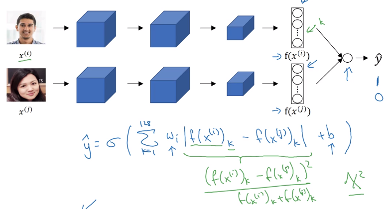
computation trick: precompute encodings of imgs in database at inference time.

II-Neural Style Transfer

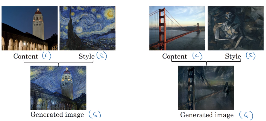
What is neural style transfer?

content image C+ style image S → generated image G

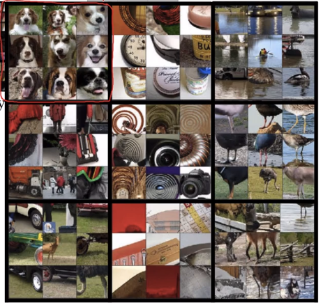
What are deep ConvNets learning?

visualize hidden units of different layers
Pick one unit in 1st layer → find the nine image patches that maximize the unit's activation.

In deeper layers: units can see larger image patches → gather nine argmax image patchs as before.

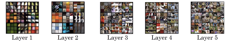
deeper layers can detect higher level shapes:
layer 3:

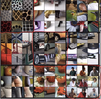
layer 4:

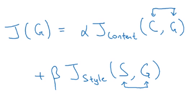
Cost Function

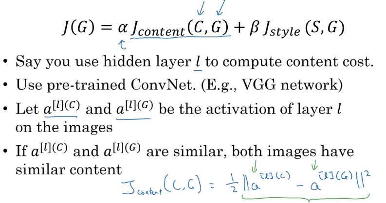
Define a cost function for the generated image.
J(G) measure how good is an image, contains two parts:

• J_content(C, G): how similar is G to C
• J_style(S, G): how similar is G to S.

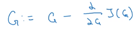
Find generated image G
(similar to embedding?)

• initialize G randomly
• Use gradient-descent to minimized J(G)

Content Cost Function

J_content(C, G)

Given a pre-trained CNN, use hidden layer l to compute J_content. The depth of l controls the level of details focuses on.

Define J_content(C, G) = difference (e.g. L2-norm) between the activation of layer l of image C and image G.

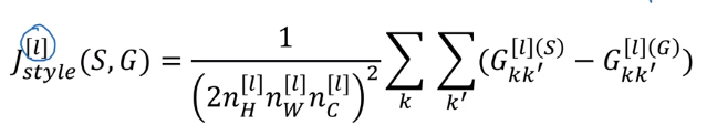
Style Cost Function

Use layer l to measure "style".
→ style defined as correlation between activations across channels.
e.g. n_C=5 channels of slices n_W * n_H.

correlation between 2 channel ~= which high-level features tend to occur / not occur together in an image.

style matrix
notation:

• a_ijk = (scalar)activation at hight=i, width=j, channel=k
• "Style matrix) G[l], (G for "Gram matrix") shape = n_C * n_C, measures how correlated any two channels are. (i.e. G[l] measures the degree to which the activations of different feature detectors in layer l vary (or correlate) together with each other.)
• G_kk' = correlation between kth and k'th channel.

:= sum_over_i_j( a_ijk * a_ijk')

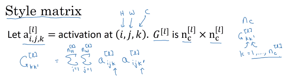
mathematically, this "correlation" is unnormalized cross-covariance (without substracting the mean).

Compute G for both the style image and generated image.
→ J_style(Gen_img, Sty_img) = difference (Frobenius norm) between G(gen) and G(sty)

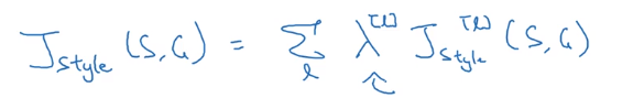
In practice, take J_style for multiple layers:

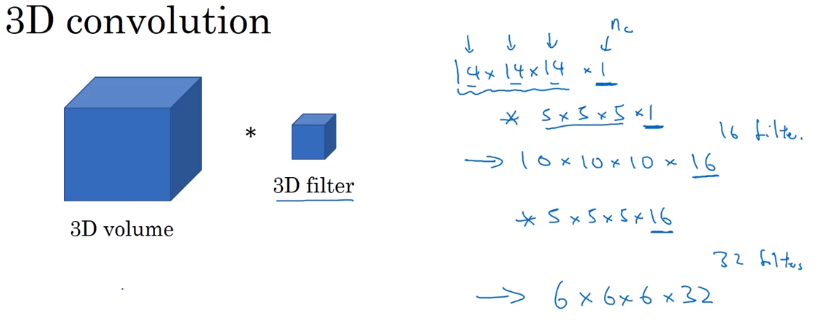
1D and 3D Generalizations

images: 2D data.
→ generalize convolution to 1D and 3D data.

1D data
e.g. EKG data (heart voltage).

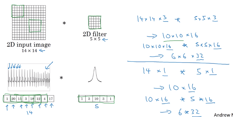
(note: most 1D data use RNN...)

3D data
have height width and depth,
e.g. C.T. data; movie date (frame by frame)
→ generalized from 2D