Computer Vision

CV with DL: rapid progress in past two years.

CV problems:

• image classification
• object detection: bounding box of objects
• neural style transfer

input features could be very high dimension: e.g. 1000x1000 image → 3 million dim input ⇒ if 1st layer has 1000 hidden units → 3 billion params for first layer...

foundamental operation: convolution.

Edge Detection Example

Motivating example for convolution operation: detecting vertical edges.

Convolve image with a filter(kernel) matrix:

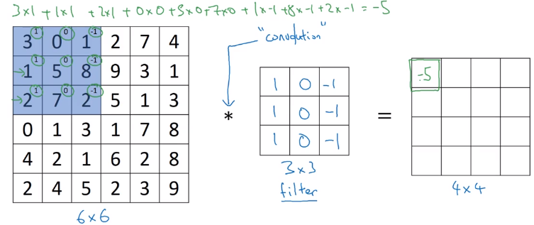
Each element in resulting matrix: sum(element-wise multiplication of filter and input image).

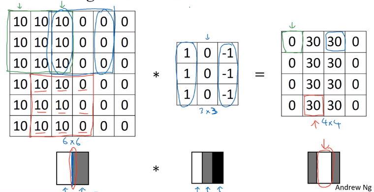
Why the filter can detect vertical edge?

More Edge Detection

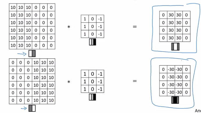
Positive V.S. negative edges:
dark to light V.S. light to dark

Instead of picking filter by hand, the actual parameters can be learned by ML.
Next: discuss some building blocks of CNN, padding/striding/pooling...

Padding

Earlier: image shrinks after convolution.
Input n*n image, convolve with f*f filter ⇒ output shape = (n-f+1) * (n-f+1)
downside:

• image shrinks on every step (if 100 layer → shrinks to very small images)
• pixels at corner are less used in the output

⇒ pad the image so that output shape is invariant.

if p = padding amount (width of padded border)
→ output shape = (n+2p-f+1) * (n+2p-f+1)

Terminology: valid and same convolutions:

• valid convolution: no padding, output shape = (n-f+1) * (n-f+1)
• same convolution: output size equals input size. i.e. filter width p = (f-1) / 2 (only works when f is odd — this is also a convention in CV, partially because this way there'll be a central filter)

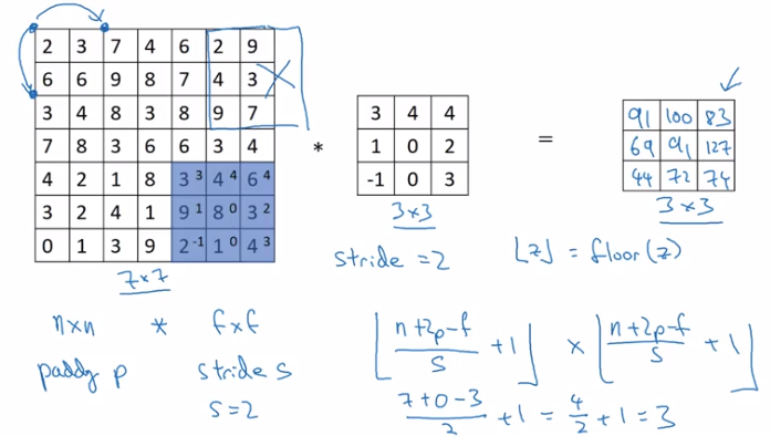
Strided Convolutions

Example stride = 2 in convolution:

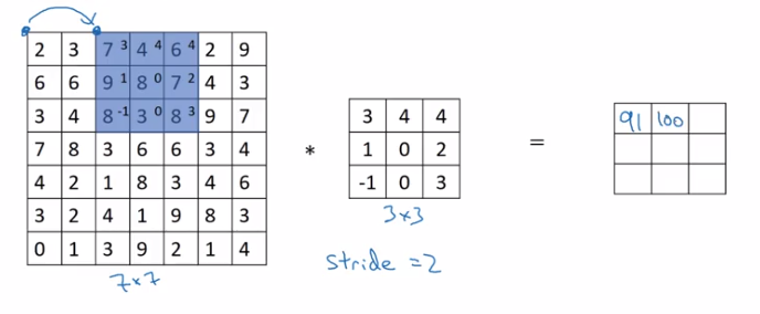
(convention: stop moving if filter goes out of image border.)

if input image n*n, filter size f*f, padding = f, stride = s
⇒ output shape = (floor((n+2p-f)/s) + 1) * (floor((n+2p-f)/s) + 1)

Note on cross-correlation v.s. convolution
In math books, "convolution" involves flip filter in both direction before doing "convolution" operation.

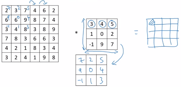
The operation discribed before is called "cross-correlation".

(Why doing the flipping in math: to ensure assosative law for convolution — (AB)C=A(BC).)

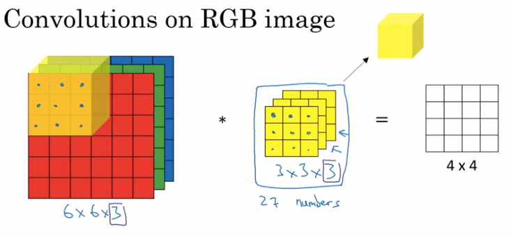
Convolutions Over Volume

example: convolutions on RGB image
image size = 663 = height * width * #channels
filter size = 333, (convention: filter's #channels matches the image)
output size = 44 (1) — output is 2D for each filter.

Multiple filters:

• take >1 filters
• stack outputs together to form an output volume.

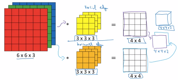
Summary of dimensions:
input shape = n*n*n_c
filter shape = f*f*n_c

filters = n_c'

⇒ output shape = (n-f+1) * (n-f+1) * n_c'

One Layer of a Convolutional Network

For each filter's output: add bias b, then apply nonlinear activation function.

One layer of a CNN:

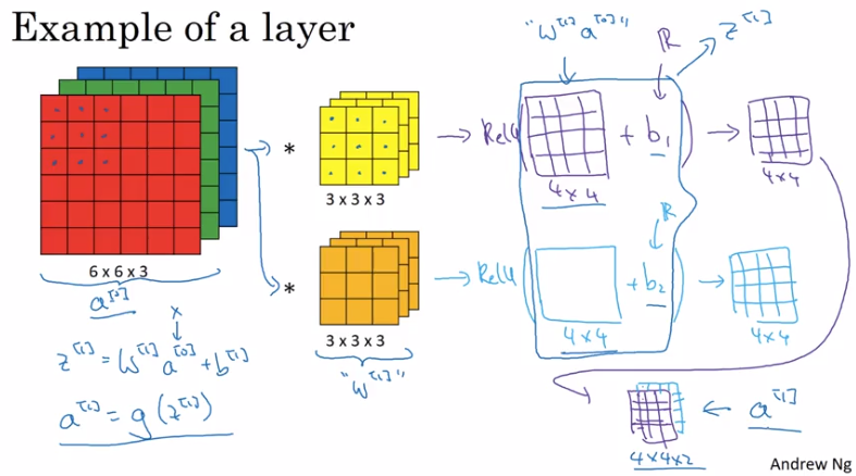
with analogy to normall NN:

• linear operation (matrix mul V.S. convolution)
• bias
• nonlinear activation
• difference: Number of parameters doesn't depend on input dimension: even for very large images.

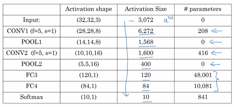
Notation summary:

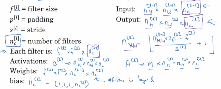
note: ordering of dimensions: example index, height, width, #channel.

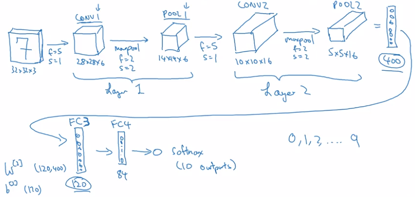
Simple Convolutional Network Example

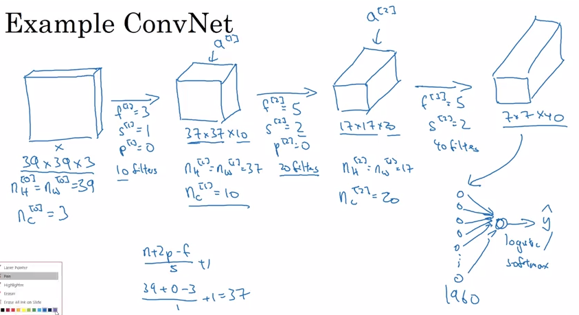
general trend: as going to later layers, image size shrinks, #channels increases.

Pooling Layers

Pooling layers makes CNN more robust.

Max pooling
divide input into regions, take max of each region.

• Hyperparams:

(common choice) filter size f=2 or 3, strid size s=2, padding p=0.

• note: no params to learn for max pooling layer, pooling layer not counted in #layers (conv-pool as a single layer)

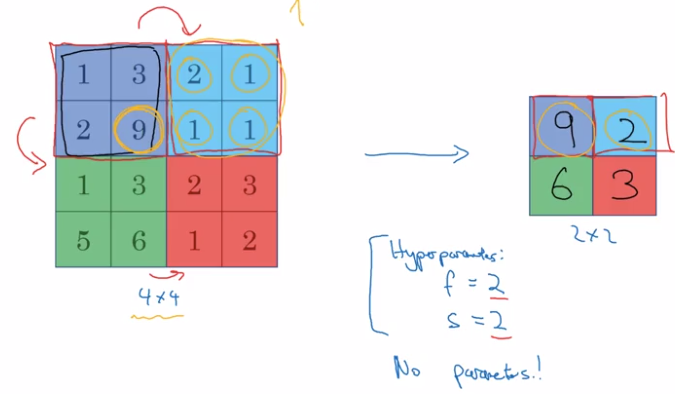
Intuition: a large number indicats a detected feature in that region → preseved after pooling.

Formula of dimension floor((n+2p-f+1)/s + 1) holds for POOL layer as well.

Output of max pooling: the same #channels as input (i.e. do maxpooling on each channel).

Average pooling
Less often used than max pooling.
Typical usecase: collapse 771000 activation into 111000.

CNN Example

LeNet-5

Why Convolutions?

2 main advantages of CONV over FC: param sharing; sparsity of connections.

Parameter sharing:
A feature detector useful in one part of img is probably useful in another part as well.
→ no need to learn separate feature detectors in different parts.

Sparsity of connections:
For each output value depends only on a small number of inputs (the pixels near that position)

• Invarance to translation...