- Mini-batch gradient descent
- Understanding mini-batch gradient descent
- Exponentially weighted (moveing) averages
- Understanding exponentially weighted averages
- Bias correction in exponentially weighted averages
- Gradient descent with momentum
- RMSprop
- Adam optimization algorithm
- Learning rate decay
- The problem of local optima
- assignment
This week: optimization algos to faster train NN, on large dataset.
Mini-batch gradient descent
batch v.s. mini-batch GD
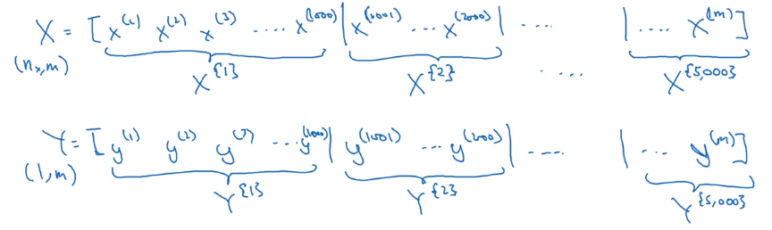
Compute J on m examples: vectorization, i.e. stacking x(i) y(i) horizontally.
X = [x(1), ..., x(m)]
Y = [y(1), ..., y(m)]
→ still slow or impossible with large m.
⇒ split all m examples into mini-batches. X^t^, Y^t^
e.g. mini batch size = 1000.
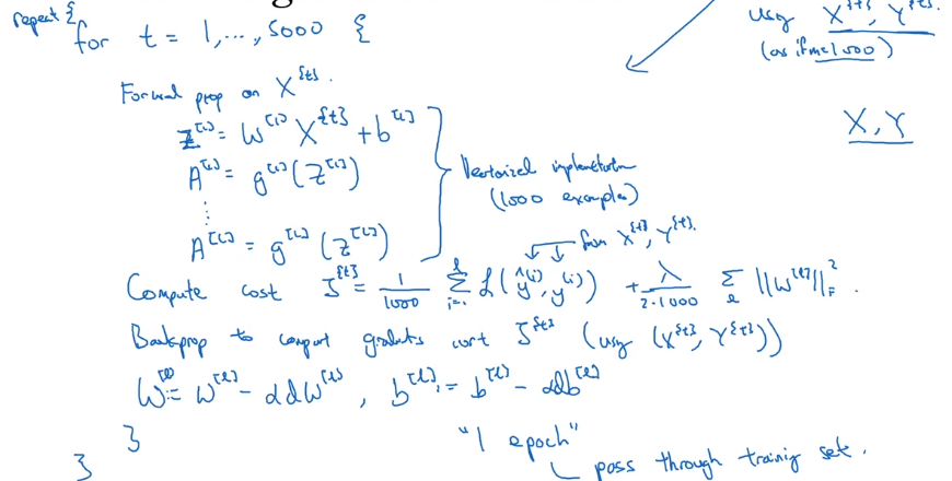
Minibatch GD:
each step, run one iteration of GD using X{t}, Y{t} instead of doing with full X, Y.
one "epoch": one pass through all training set
Understanding mini-batch gradient descent
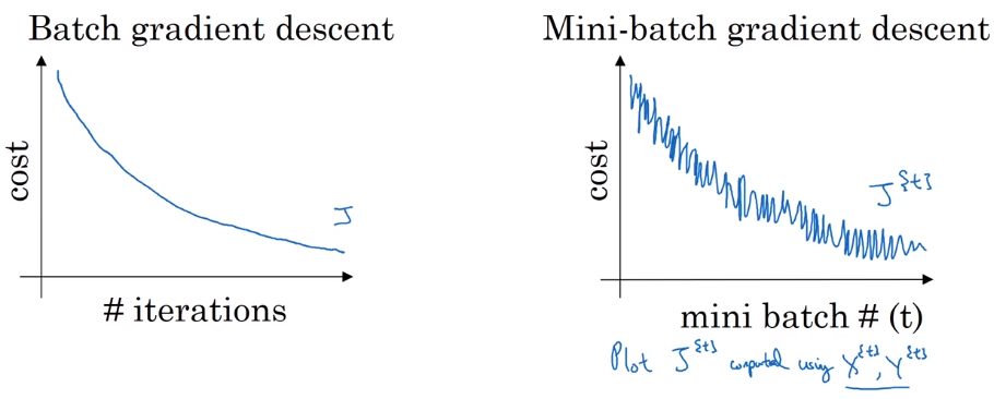
with batch-GD: each iteration will decrease cost function.
in mini-batch: cost J^t^ is computed on different dataset — noisy.
How to choose minibatch size
-
extreme 1: minibatch size = m → batch GD
coverge fastest in each iter (but too long time or impossible per iter)
-
extreme 2: minibatch size = 1 → stochastic GD
noisy, never coverge, (but loose all vectorization speedup)
Guidelines on choosing batch size:
- small training set (m<2000) → just batch size
-
otherwise:
typical minibatch size = 64/128/256/512 (make sure minibatch size fits in CPU/GPU memory)
Exponentially weighted (moveing) averages
In fact, exp-weighted-avg is an non-parametric estimator/smoother of a series of vlaues.
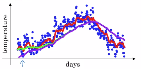
example: Temperature over the year
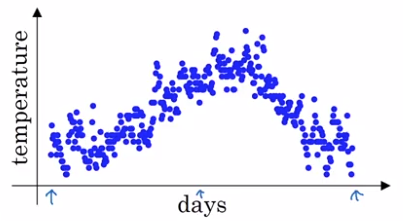
→ use a exp-weighted moving average to model this:
theta[t] = temperature at day t, t = 1,2,3,...
v[t] = averaged(smoothed) estimate of theta, t = 0,1,2,3,...
exp-weighted average: recursivly compute v[t].
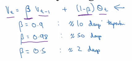
v[0] = 0, v[t] = 0.9 * v[t-1] + 0.1 * theta[t]
(param: beta = 0.9)
⇒ v[t] ~= average of theta[t] over the last 1/(1-beta) days. (c.f. next section)
Understanding exponentially weighted averages

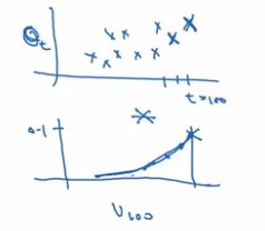
Understanding the math of exp-weighted-average:
→ unroll the recursive formula:
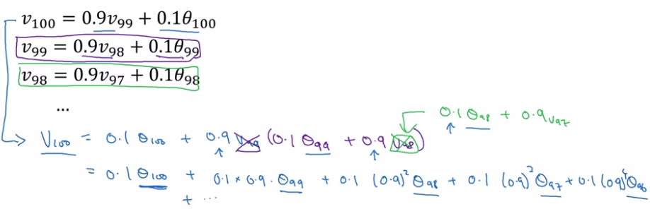
⇔ v[100] = a convolution of theta[t-100:t] and a exp-decaying function:
A small trick on estimating exps:
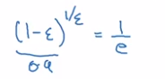
That's why in previous section, we say this formula ~= averaging over last 1/(1-beta) (=1/epslon) days' theta.
e.g. theta[t-10]'s weight is 0.9 ^ 10 ~= 1/e ~= 0.35, i.e. after 10 days, the weight of theta[t-10] is decayed to ~< 1/3.
Advantage to just computing moving window averages: in implementation, only keep updating a single variable v_theta — very small memory usage.
Bias correction in exponentially weighted averages
To make exp-weighted averages more accurate by bias correction.
Problem with previous implementation in initial phase:
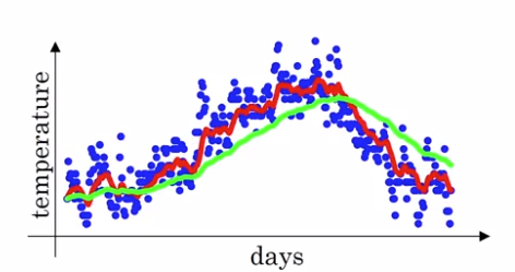
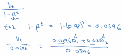
- v[0] = 0, beta = 0.98
- v[1] = 0.980 + 0.02 * theta[1] ⇒ v[t] starts lower than theta. *(purple curve VS green curve)
⇒ Correction:
take v[t] / (1 - beta^t) instead of v[t].
In practice: most people don't bother to implement bias correction — just wait for the initial phase to warm up...
Gradient descent with momentum
GD with momentum:
- almost always faster than normal GD
- in short: compute exp-weighted-avg of the gradients as gradient to use
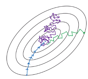
example: if contour of loss is an ellipse, can't use too large step in GD, and oscillate. → average of steps will be faster.
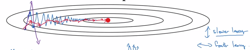
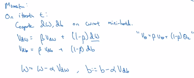
GD momentum:
Use exp-weighted-avg of dW (V_dW) and of db (V_db). — smooth out oscillation steps of normal GD.
update params with the averaged value V_dW, V_db.
Why the name "momentum": rolling down a ball in a bowl
dW/db: ~accelation
V_dW/B_db: ~velocity at current time (this is why the smoothing average is called 'v')
beta: ~friction
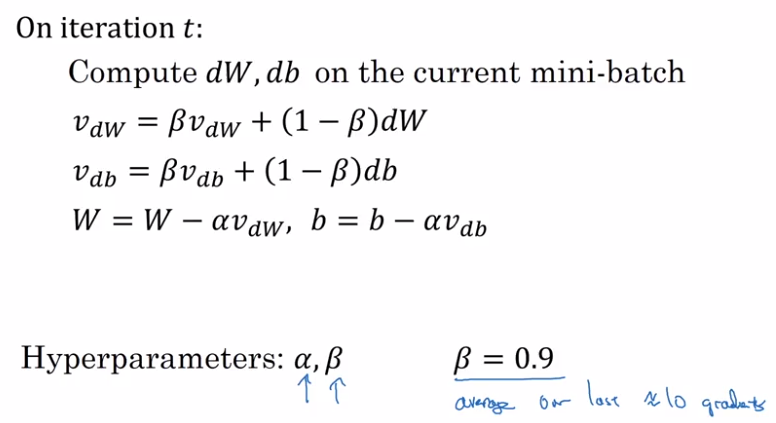
in practice:
- beta=0.9 works well for most cases
- no bias correction implemented
- can use beta = 0 → ~V_dW is scaled by 1/(1-beta) → use a scaled alpha then.
⇒ less intuitive, and couples the tuning of alpha and beta
RMSprop
"Root-Mean-Square-prop".
- also for speedup GD
-
in short:
S = exp-weighted-avg of gradient squared (that's why call param beta2);
when updating params(W,b), scale dW,db by sqrt of S.dW / sqrt(S_dW)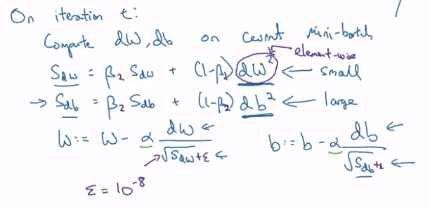
example: ellipse contour, want slow rate in
bdirectrion and fast rate inwdirection.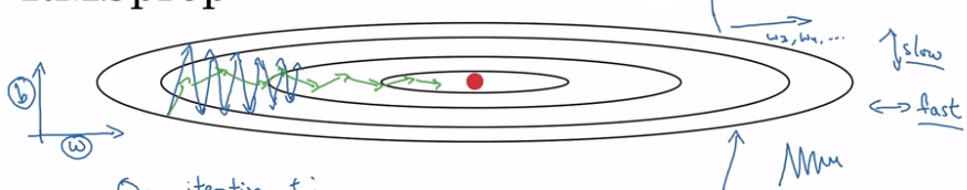
⇒ for each step (dW, db) = gradient of current minibatch:
-
db large, dW small
→ update w by dW/sqrt(S_dW), ⇔ larger step in W direction
→ db/sqrt(S_db) ⇔ smaller step in b direction → damping out oscillations in b direction
Adam optimization algorithm
"Adaptive Moment-estimation"
- A combination of RMSprop and momentum.
- Proved to work well for a varity of problems.
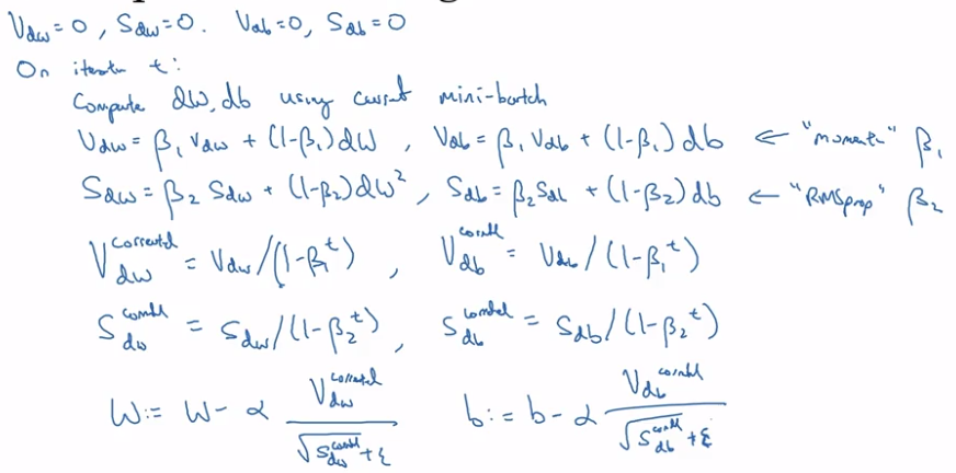
Algo:
- maintain both V_dW, V_db (hyper-param=beta1) and S_dW, S_db (hyper-param=beta2)
- implement bias correction: V_corrected, S_corrected — divid by (1-beta^t)
- param update (W, b):
V / sqrt(S)
hyperparameters:
- alpha: learning rate, needs tuning
- beta1: usually 0.9
- beta2: usually 0.999
- epsilon: 10e-8 (not important)
Learning rate decay
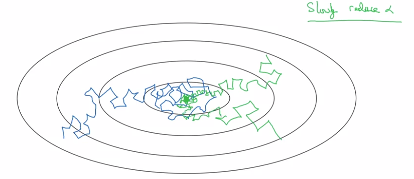
slowly reduce learning rate.
In minibatch with fixed learning rate: will never converge.
⇒ decay learning rate → oscillating around a smaller region of optima.
Implementation:
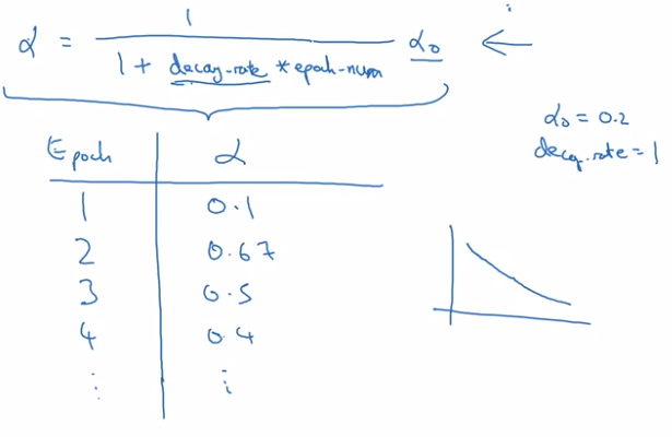
- 1 epoch = 1 pass through whole data.
- decay learning rate alpha after each epoch (hyper-param decay-rate):
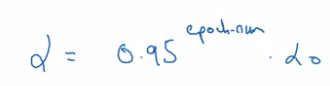
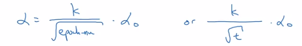
other decay method:
- exponentially decay alpha:
- sqrt of epoch_num:
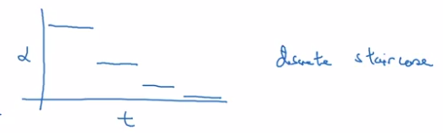
- discrete staircase:
- manual decay: when training takes long time
The problem of local optima
low-dimention optimas:
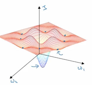
This gives wrong intuition, in practice (high-dim), most 0-gradient points are saddle points.
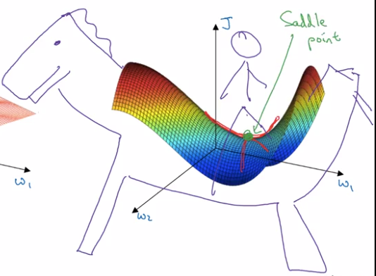
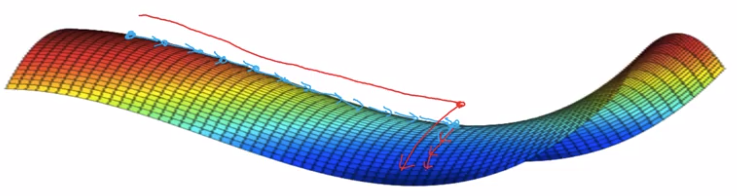
plateau: region where gradient close to 0 for long time.
take-away:
- unlikely to stuck in bad local optima: D dimentional → ~2^(-D) of chance.
- plateaus can make learning slow → use momentum/RMSprop/Adam to speedup training.
assignment
implementing mini-batch GD:
shuffle data (note: X and Y's columns are sync-ed!):
permutation = list(np.random.permutation(m))
        shuffled_X = X[:, permutation]
        shuffled_Y = Y[:, permutation].reshape((1,m))
→ partition data:
kth mini batch:
mini_batch_X = shuffled_X[:, k*mini_batch_size:(k+1)*mini_batch_size]
     mini_batch_Y = shuffled_Y[:, k*mini_batch_size:(k+1)*mini_batch_size]
detail: when m % minibatch_size != 0: handle last batch (smaller than a regular batch)
Part 6 of series «Andrew Ng Deep Learning MOOC»:
- [Neural Networks and Deep Learning] week1. Introduction to deep learning
- [Neural Networks and Deep Learning] week2. Neural Networks Basics
- [Neural Networks and Deep Learning] week3. Shallow Neural Network
- [Neural Networks and Deep Learning] week4. Deep Neural Network
- [Improving Deep Neural Networks] week1. Practical aspects of Deep Learning
- [Improving Deep Neural Networks] week2. Optimization algorithms
- [Improving Deep Neural Networks] week3. Hyperparameter tuning, Batch Normalization and Programming Frameworks
- [Structuring Machine Learning Projects] week1. ML Strategy (1)
- [Structuring Machine Learning Projects] week2. ML Strategy (2)
- [Convolutional Neural Networks] week1. Foundations of Convolutional Neural Networks
- [Convolutional Neural Networks] week2. Deep convolutional models: case studies
- [Convolutional Neural Networks] week3. Object detection
- [Convolutional Neural Networks] week4. Special applications: Face recognition & Neural style transfer
- [Sequential Models] week1. Recurrent Neural Networks
- [Sequential Models] week2. Natural Language Processing & Word Embeddings
- [Sequential Models] week3. Sequence models & Attention mechanism
Disqus 留言