This week: logistic regression.

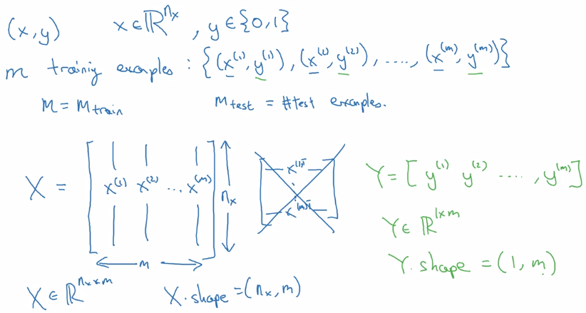
Binary Classification & notation

ex. cat classifier from image image pixels: 64x64x3 ⇒ unroll(flatten) to a feature vector x dim=64x64x3=12288:=n (input dimension)

notation

• superscript (i) for ith example, e.g. x^(i)
• superscript [l] for lth layer, e.g. w^[l]
• m: number of data
• n_x: input dimension, n_y: output dimension.
• n_h^[l]: number of hidden units for layer l.
• L: number of layers
• X: dim=(n_x,m), each column is a training example x^(i).
• Y: dim=(1,m), one single row matrix.

Logistic Regression as a Nueral Network

Logistic Regression

dim(x) = n_x parameters: w (dim=n_x) , b (dim=1) (alternative notation: adding b to w → add x_0 = 1 to feature x. → will NOT use this notation here keeping w and b separate make implementation easier )

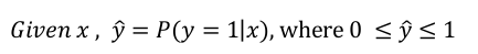
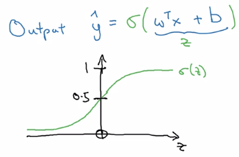
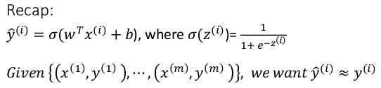
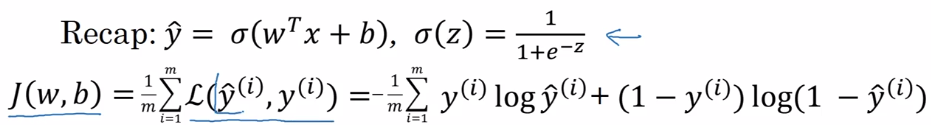
linear regression: y_hat = w^T*x + b logistic regssion: y_hat = sigmoid(w^T*x + b) sigmoid function: S-shaped function sigmoid(z) = 1 / ( 1 + e^-z) z large → sigmoid(z) ~= 1 z small → sigmoid(z) ~= 0

Logistic Regression Cost Function

To train model for best parameters (w, b), need to define loss function.

y_hat: between (0,1) training set: {(x^(i), y^(i)))), i = 1..m} want: y_hat(i) ~= y(i)

Loss function L(y_hat, y): on a single training example (x, y)

• square error: L(y_hat, y) = (y_hat - y)^2/2
  • ⇒ not convex, GD not work well, uneasy to optimize
• loss function used in logistic regression:

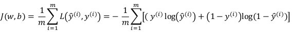
L(y_hat, y) = -[ylog(y_hat) + (1-y)log(1-y_hat)]

• convex w.r.t. w and b
• when y = 1, loss = -log(y_hat) → want y_hat large → y_hat ~=1
• when y = 0, loss = -log(1-y_hat) → want y_hat small → y_hat ~=0

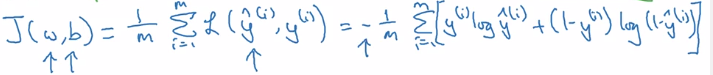
Cost function J(w,b): average on all training sets, only depends on parameters w, b

Gradient Descent

⇒ minimize J(w,b) wrt. w and b

• J(w,b) is convex ⇒ gradient descent
• Initialization: for logistic regression, any init works because of convexity of J, usually init as 0

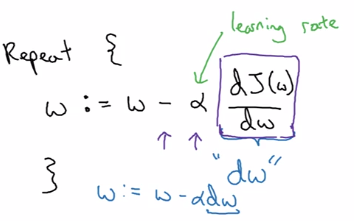
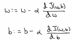
Gradient descent:

• alpha = learning rate
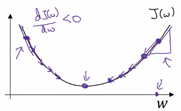
• derivative dJ(w)/dw

~= slope of function J at point w ~= direction where J grows fastest at point w denote this as 'dw' in code

• algo: 'take steepest descent'
  • from an init value of w_0
  • repeatedly update w until converge w := w - alpha*dw

In the case of logistic regression, >1 params (w and b) to update:

Intuitions about derivatives: f'(a) = slope of function f at a .

Computation Graph

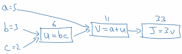
example: function J(a,b,c) = 3(a+b*c)

Forward propagation: compute J(a,b,c) value:

• internal u := b*c
• internal v := a+u
• J = 3 * v

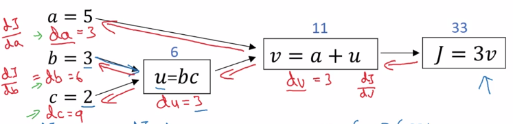
Backward propagation: compute derivatives dJ/da, dJ/db, dJ/dc:

• J = 3*v → compute dJ/dv
• v = a + u → compute dv/da, dv/du
• u = bc → compute du/db, du/dc

⇒ chain rule: dJ/da is multiplying the derivatives along the path from J back to a

• dJ/da = dJ/dv * dv/da
• dJ/db = dJ/dv * dv/du * du/db

• dJ/dc = dJ/dv * dv/du * du/dc

• In code: denote 'dvar' as d(FinalOutput)/d(var) for simplicity. i.e. da = dJ/da, dv = dJ/dv, etc.

Logistic Regression Gradient Descent (&computation graph)

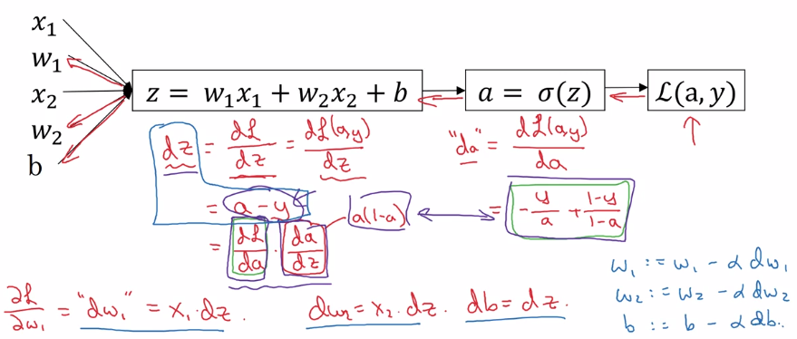
logistic regression loss(on a single training example x,y) L. as computation graph:

• z = wx + b
• a := sigmoid(z) (=y_hat, 'logit'?)
• loss function L(a,y) = - [y(loga) + (1-y)log(1-a)]

Gradient Descent on m Examples

cost function, i.e. on all training sets.

J(w,b) = avg{L(x,y), for all m examples} → by linearity of derivative: dJ/dw = avg(dL/dw), just average dw^(i) over all indices i.

In implementation: use vectorization as much as possible, get rid of for loops.

Python and Vectorization

Vectorization

avoid explicit for-loops whenever possible e.g. z = w^T * x + b in numpy: z = np.dot(w, x) + b ~300 times faster than explicit for loop

more examples: u = A*v matrix multiplication → u = np.dot(A, v) note: A * v would element-wise multiply u = exp(v) element-wise operation: exponential/log/abs/... → u = np.exp(v) / np.log(v) / np.abs(v) / v**2 / 1/v

Vectorizing Logistic Regression

implementation before: two for-loops( 1 for each training set, 1 for each feature vector).

• training input X = [x(1), ... , x(m)], X.dim = (n_x, m)
• weight w^T = [w_1, ... , w_nx], w.dim = (n_x, 1)

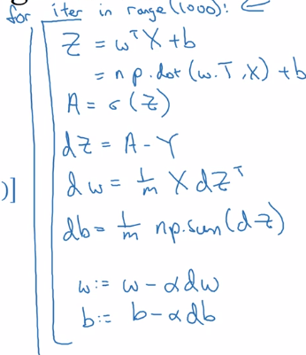
Fwd propagation
z(i) = w^T * x(i) + b, i = 1..m, → Z := [z(1)...z(m)] = w^T * X + [b...b], Z.dim = (1, m), stack horizentally → Z = np.dot(w.T, X) + b (scalar b auto broadcasted to a row vector) a(i) = sigmoid( z(i) ) = y_hat(i) → A := [a(1)...a(m)] = sigmoid(Z), sigmoid is vectorized

Bkwd propagation: gradient computation
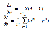
dz(i) = a(i) - y(i) → stack horizentally: Y = [y(1)...y(m)] dZ := [dz(1)...dz(m)] = A - Y graidents: dw = sum( x(i) * dz(i) ) / m, dw.dim = (nx, 1) db = sum( dz(i) ) / m → db = 1/m * np.sum(dZ) dw = 1/m * X*dz^T

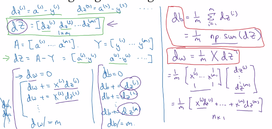
efficient back-prop implementation:

Broadcasting in Python

example: calculate percentage of calories from carb/protein/fat for each food — without fooloop

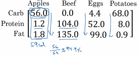
two lines of numpy code: A = np.array([[...]..]) # A.dim = (3,4) cal = A.sum(axis=0) # total calories percentage = 100 * A / cal.reshape(1,4) # percentage.dim = (1,4)

• axis=0→ sum vertically, axis=1 → sum horizentally

• reshape(a,b) → redundant here, just to make sure shape correct, reshape call is cheap.
• A / cal → (34 matrix) / (14 matrix) → broadcasting

more broadcasting examples:

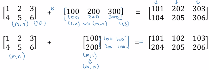
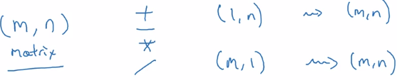
General principle: computing (m,n) matrix with (1,n) matrix ⇒ the (1,n) matrix is auto expanded to a (m,n) matrix by copying the row m times, to match the shape, calculate element-wise

A note on python numpy vectors

flexibility of broadcasting: both advantage and weakness. example: adding column vec and a row vec → get a matrix instead of throwing exceptions. >>> a array([1, 2, 3]) >>> b array([[1], [2]]) >>> a + b array([[2, 3, 4], [3, 4, 5]])

Tips and trick to eliminate bugs

avoid rank-1 array:
a.shape = (x,) this is neither row nor column vector, have non-intuitive effects. >>> a = np.array([1,2,3]) >>> a.shape (3,) # NOT (3,1) >>> a.T array([1, 2, 3]) >>> np.dot(a, a.T) # Mathematically would expact a matrix, if a is column vec 14 >>> a.T.shape (3,)

⇒ do not use rank-1 arraies, use column/row vectors >>> a2 = a.reshape((-1, 1)) # A column vector -- (5,1) matrix. >>> a2 array([[1], [2], [3]]) >>> a2.T array([[1, 2, 3]]) # Note: two brackets!

add assertions
assert(a.shape == (3,1))

Explanation of logistic regression cost function (optional)

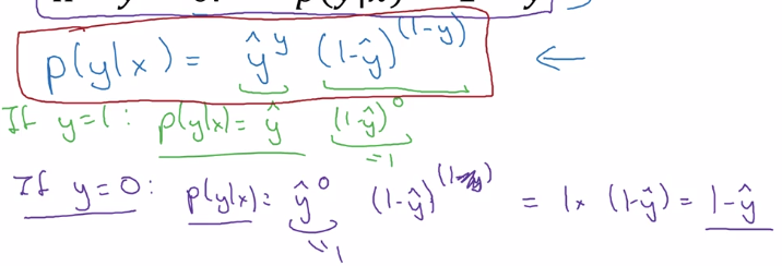
Justisfy why we use this form of cost function: y_hat ~= chance of y==1 given x want to express P(y|x) using y_hat and y P(y|x) as func(y, y_hat) at different values of y:

• if y = 1: P(y|x) = P(y=1|x) = y_hat
• if y = 0: P(y|x) = P(y=0|x) = 1 - y_hat

⇒ wrap the two cases in one single formula: using exponent of y and (1-y)

⇒ take log of P(y|x) ⇒ loss function (for a single training example)

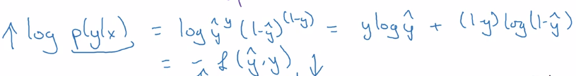
⇒ aggregate over all training examples i = 1..m: (assume: data are iid) P(labels in training set) = multiply( P(y(i)|x(i) ) take log → log(P(labels in training set)) = sum( log P(y(i)|x(i) ) = - J maximizing likelihood = minimizing cost function

Assignments

python / numpy basics

• np.reshape() / np.shape
• calculate norm: np.linalg.norm()

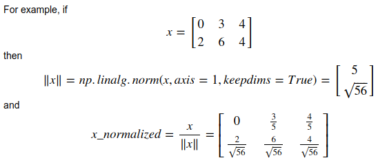
• keepdims=True:

axes that are reduced will be kept (with size=1)

  >>> a
  array([[ 0.01014617,  0.08222027, -0.59608242],
        [-0.18495204, -1.50409531, -1.03853663],
        [ 0.03995499, -0.67679544,  0.11513247]])
  >>> a.sum(keepdims=1)
  array([[-3.75300795]])
  >>> a.sum()
  -3.7530079538833663

• broadcasting
• softmax:

softmax for row vec: x.shape = (1,n), x = [x1,...xn] y = softmax(x), y.shape = (1,n), yi = exp(xi) / sum( exp(xi) ) softmax for matrix X.shape = (m,n) Y = softmax(X) = [softmax(row-i of X)], Y.shape = (m, 1)

Logistic Regression with a Neural Network mindset

• input preprocessing

input dataset shape = (m, num_px, num_px, 3) → reshape to one column per example, shape = (num_pxnum_px3, ~~m~~) → center & standardize data: x' = (xi - x_mean) / std(x), but for images: just divide by 255.0 (max pixel value), convenient and works almost as well.

• params initialization

For logistic regression (cost function convex), just init to zeros is OK. w = np.zeros((dim,1)) b = 0.0

• Fwd prop: compute cost function

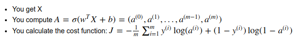
input X (shape = nx*m, one column per example)→ logits Z → activations A=sigmoid(Z)→ cost J

• Bkwd prop

• Optimization

gradient descent: w := w - alpha*dw

• Predict: using learned params

Yhat = A = sigmoid(wT * X + b)